Analysis the customer action with RFM method.
Using language and Tools
Python, Pandas-profiling, Pandas, SKlearn, Matplotlib
Goal of this project
The objective of this project is to analyze e-commerce customer action data and classify customers based on the characteristics identified in the data.
Dataset Description
This data is archived from this link
Link from “archive.ics.uci.edu”.
This is a transnational data set which contains all the transactions occurring between 01/12/2010 and 09/12/2011 for a UK-based and registered non-store online retail. The company mainly sells unique all-occasion gifts. Many customers of the company are wholesalers.
Data Description
| Variable Name | Role | Type | Description |
|---|---|---|---|
| InvoiceNo | ID | Categorical | 6-digit integral number uniquely assigned to each transaction. If this code starts with letter ‘c’, it indicates a cancellation |
| StockCode | ID | Categorical | 5-digit integral number uniquely assigned to each distinct product |
| Description | Feature | Categorical | product name |
| Quantity | Feature | Integer | the quantities of each product (item) per transaction |
| InvoiceDate | Feature | Date | the day and time when each transaction was generated |
| UnitPrice | Feature | Continuous | product price per unit |
| CustomerID | Feature | Categorical | 5-digit integral number uniquely assigned to each customer |
| Country | Feature | Categorical | the name of the country where each customer resides |
EDA with pandas_profiling
Exploratory Data Analysis (EDA) is a crucial step in the data analysis process, allowing us to understand the structure and characteristics of our dataset. pandas_profiling is a powerful Python library that automates much of the EDA process, providing comprehensive insights into the dataset.
“Pandas_profiling” Overview
Pandas_profiling generates an interactive HTML report that includes various statistics, visualizations, and summaries of the dataset. It’s particularly helpful for quickly grasping the key aspects of the data without having to write extensive code.
Here is the result from pandas profiling library.
pandas_profiling simplifies the EDA process by automating the generation of detailed reports. However, it’s crucial to complement this automated analysis with domain-specific knowledge and additional exploratory techniques for a comprehensive understanding of the data.
Data Rediness Check
1. Remove duplicated data
When dealing with datasets, ensuring data integrity is important. In this step, I found potential duplicates in the dataset.
   df = df.drop_duplicates().reset_index(drop=True)
   print("After drop, Duplicated value :", len(df[df.duplicated()]))
After drop, Duplicated value : 0
After executing this process, we observe that there are no remaining duplicated values in the dataset (Duplicated value: 0), indicating a cleaner and more reliable dataset.
2. EDA of the dataset
   list_cast_to_object = ["CustomerID"]
   for column_name in list_cast_to_object:
   df[column_name] = df[column_name].astype(object)
Visualizing and understanding the dataset is a crucial step in data analysis. The graph above provides a snapshot of key insights obtained through EDA.
To enhance the analysis further, we identify that casting the CustomerID column to an object type can be beneficial for certain operations.
This conversion allows for more effective categorical analysis and aligns with the nature of customer identifiers.
3. Devide the dataset into numeric data and categorical data.
Understanding the data types within the dataset is vital process. Here, we categorize columns into numeric and categorical types.
   # make list of categorical data
   list_categorical_columns = list(df.select_dtypes(include=['object']).columns)

   # make list of numeric data
   list_numeric_columns = list(df.select_dtypes(include= ['float64','int64']).columns)

   print("Length of data: ",len(df))
   print("Length of columns: ",len(df.columns))
   print("categorical columns:",len(list_categorical_columns))
   print("numerical columns:",len(list_numeric_columns))
The provided statistics give us a comprehensive view of the dataset, with information on data length, column count, and the distribution between categorical and numerical columns. This segmentation sets the stage for tailored analysis approaches based on the nature of the data.
These initial data preparations and exploratory steps lay the foundation for more in-depth analyses and insights into the dataset.
4. Remove the useless column
Description column isn’t used in this analysis. To prevent memory leakage, I remove the “description” column.
   df = df.drop(["Description"], axis=1)
   list_categorical_columns.remove("Description")
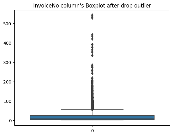
5. Remove the Outlier of each column.
To enhance the analytical utility, I aim to remove outliers from the box plot of the ‘InvoiceNo’ column, as some data points appear to be outliers. To identify and assess the outliers for removal, I will inspect the data points with a ‘max’ value of 1114 in the ‘InvoiceNo’ column using the .describe() function. This will provide insight into the specific data contributing to the outliers.
   df_invoiceno_count = df.groupby("InvoiceNo").count()["StockCode"]
   no_invoice_max = df_invoiceno_count[df_invoiceno_count > 1114]
   print(no_invoice_max.index[0])
   df[df.InvoiceNo == no_invoice_max.index[0]]
Upon inspecting the data, it is evident that the outliers have NaN values in the ‘CustomerID’ column. To address this, I applied the dropna function and reset the index. The resulting data was then visualized using a box plot, as shown below.
Categorical Data Pattern Analysis
1. Sales invoices by StockCode
   no_stockcode_buy = df.groupby("StockCode").count()["InvoiceNo"]
   no_stockcode_buy.sort_values(ascending=False)
The trend of the no_stockcode_buy data is as follows:
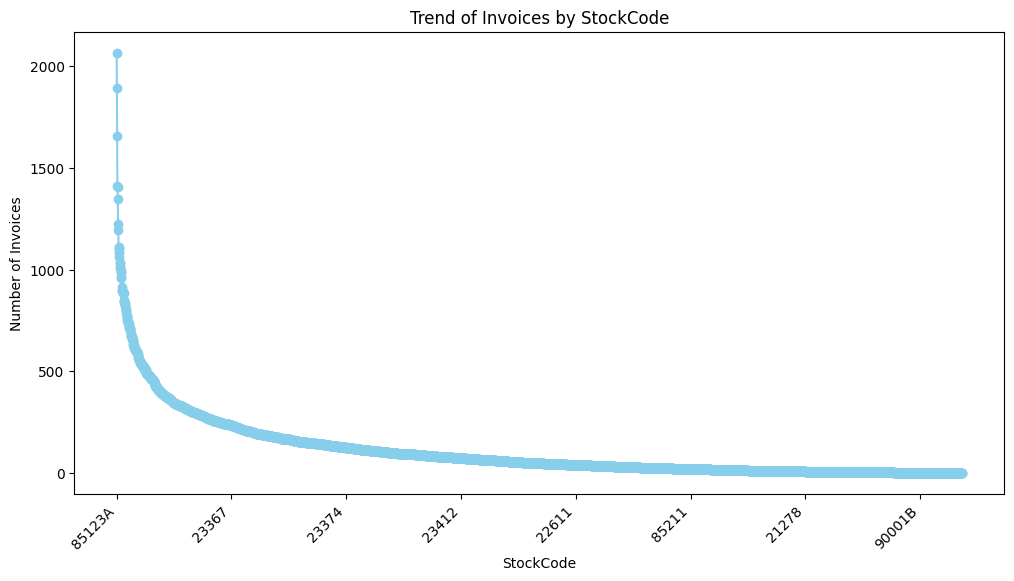
As you can see from the chart, some items are purchased by a large number of customers, while the majority of items have fewer instances of customer purchases. However, for this column, no additional transformations seem necessary.
2. Purchase rate by Day of the Week
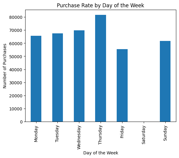
As observed in the chart, Thursday appears to be the day with the highest sales. The absence of data on Saturday suggests two possibilities: either there are no invoices issued on Saturdays, or there is a potential data contamination issue.
3. Purchase rate by Month
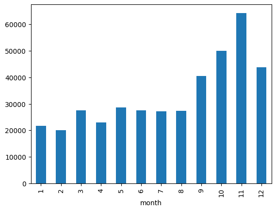
The chart depicts the monthly trend of invoice issuances. It is speculated that this store deals with a significant number of seasonal products, particularly selling a considerable amount during the winter months.
4. Purchase rate by hour
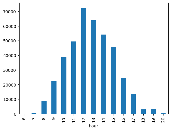
The chart illustrates the temporal trend of invoice issuances throughout the day, indicating that customers tend to place orders around lunchtime at this establishment.
5. Purchase rate by Country
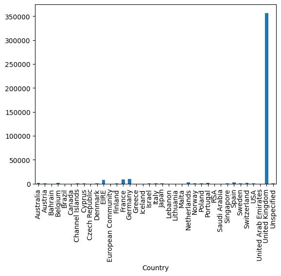
The chart comparing purchase counts by country highlights a significant dominance of orders from the UK, with only marginal orders from neighboring EU countries. If there are plans for global expansion, it might be worthwhile to consider initiatives in France or Germany, given their relatively lower order counts but potential for market growth.
Numerical Data Pattern Analysis
1. Numeric data .describe()
This is the .describe() data of Numeric columns.
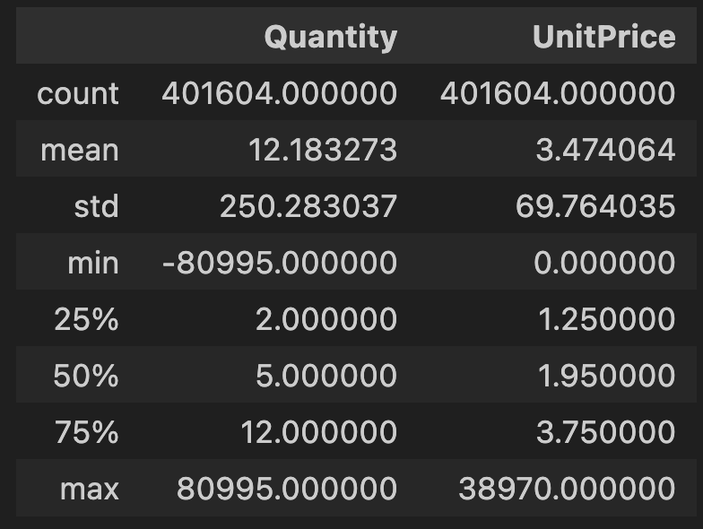
Upon examining the describe table, there is a noticeable anomaly in the data. The ‘Quantity’ column has a minimum value that is negative, indicating refund amounts, as mentioned earlier. Since refunds are deemed irrelevant for this task, the decision is made to remove these data points.
df = df[df.Quantity > 0]
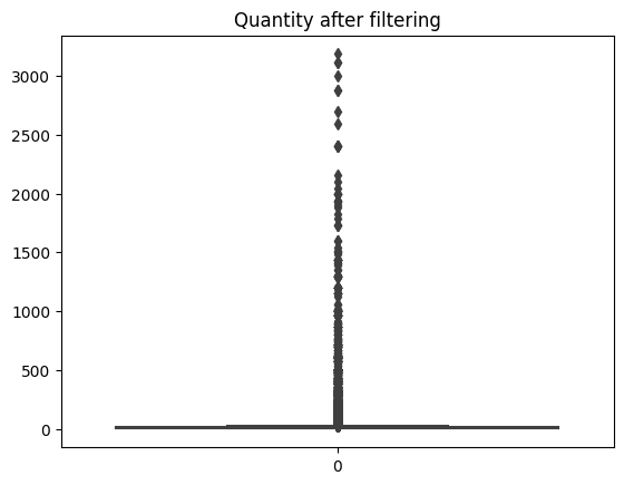
2. Quantity column
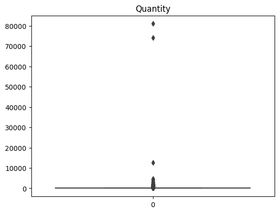
This is a box plot of the ‘Quantity’ column from numeric data. While regular products typically show order quantities of less than 10,000, some data points are treated as outliers due to extremely high quantities.
   # filtering Quantity above 3500
   df = df[df.Quantity < 3500]
Feature Engineering
I’m creating features for RFM (Recency, Frequency, Monetary) analysis, which is a powerful method for segmenting and understanding customer behavior.
1. Recency
“Recency” refers to a concept where the proximity of the purchase date is the basis for scoring, with a higher score assigned to dates closer to the present.
   # Grouping the DataFrame by customer ID and finding the maximum invoice date for each customer
   df_customer_last_date = df.groupby("CustomerID").agg(max)["InvoiceDate"].reset_index()

   # Calculating recency by subtracting the maximum invoice date from each customer
   df_customer_last_date["recency"] = (df_customer_last_date["InvoiceDate"] - df["InvoiceDate"].max()).dt.days

   # Creating a new DataFrame with recency information,and dropping the redundant InvoiceDate
   df_recency = df_customer_last_date.drop(columns=["InvoiceDate"])
2. Frequency
“Frequency” pertains to the number of purchases per customer, and a higher score is assigned to individuals who make purchases more frequently.
   df_frequency = df[["CustomerID", "InvoiceNo"]].drop_duplicates().groupby("CustomerID").count().reset_index()

   df_frequency.rename(columns = {'InvoiceNo':'frequency'}, inplace = True)
3. Monetary
“Monetary” is a criterion where a higher score is assigned based on the total purchase amount, with more substantial purchases resulting in a higher score.
   df["monetary_row"] = df["Quantity"] * df["UnitPrice"]

   non_datetime_columns = df.select_dtypes(exclude=['datetime64']).columns

   df_monetary = df.groupby("CustomerID")[non_datetime_columns].agg(sum)["monetary_row"].reset_index()

   df_monetary.rename(columns = {'monetary_row':'monetary'}, inplace = True)
4. RFM score
   # Make a new dataframe with three dimension
   df_rfm = df_recency.merge(df_frequency, on="CustomerID").merge(df_monetary, on="CustomerID")

   # Calculate N-tile of each criteria
   df_rfm["recency_ntile"] = pd.qcut(df_rfm["recency"],5, labels=[1,2,3,4,5])

   df_rfm["frequency_ntile"] = pd.qcut(df_rfm["frequency"].rank(method='first'), 5, labels=[1,2,3,4,5])

   df_rfm["monetary_ntile"] = pd.qcut(df_rfm["monetary"],5, labels=[1,2,3,4,5])
5. Scaling the score
   # Make a new feature for clustering
   df_rfm_clustering = df_rfm.copy()
   df_rfm_clustering = df_rfm_clustering[["CustomerID","recency", "frequency", "monetary"]]

   # Min-max scaling
   scaler = MinMaxScaler()
   list_scaling = ["recency", "frequency", "monetary"]
   df_rfm_clustering.loc[:, list_scaling] = scaler.fit_transform(df_rfm_clustering[list_scaling])
6. Huristic RFM analysis
   df_heuristic_rfm =df_rfm.groupby(["recency_ntile","monetary_ntile","frequency_ntile"]).agg(np.mean).reset_index()

   # Select the VIP customer
   df_rfm[(df_rfm.recency_ntile == 5) & (df_rfm.monetary_ntile == 5) & (df_rfm.frequency_ntile == 5)]
   # => 348 customers

   # Customers who made frequent purchases in the past but have reduced their buying activity recently.
   df_rfm[(df_rfm.recency_ntile == 3) & (df_rfm.monetary_ntile == 5) & (df_rfm.frequency_ntile == 5)]
7. K-means analysis using RFM
To determine the optimal value of K in K-means clustering, one important aims to find the Optimal K. This involves evaluating different values of K and selecting the one that results in the most meaningful and well-defined clusters. Common methods for finding the optimal K include the Elbow Method, Silhouette Score, and Gap Statistics. These techniques help identify the number of clusters that best captures the underlying patterns in the data.
    sum_of_squared_distances = []
    K = range(2,20)
    for k in K:
     km = KMeans(n_clusters=k)
     km = km.fit(df_rfm_clustering.drop("CustomerID", axis=1))
     sum_of_squared_distances.append(km.inertia_)
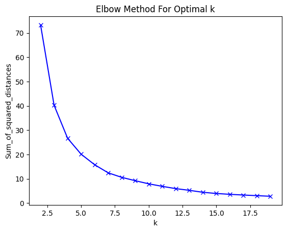
This chart indicates that choosing a value between 5 and 7 for k would be appropriate. I have decided to opt for k = 6.
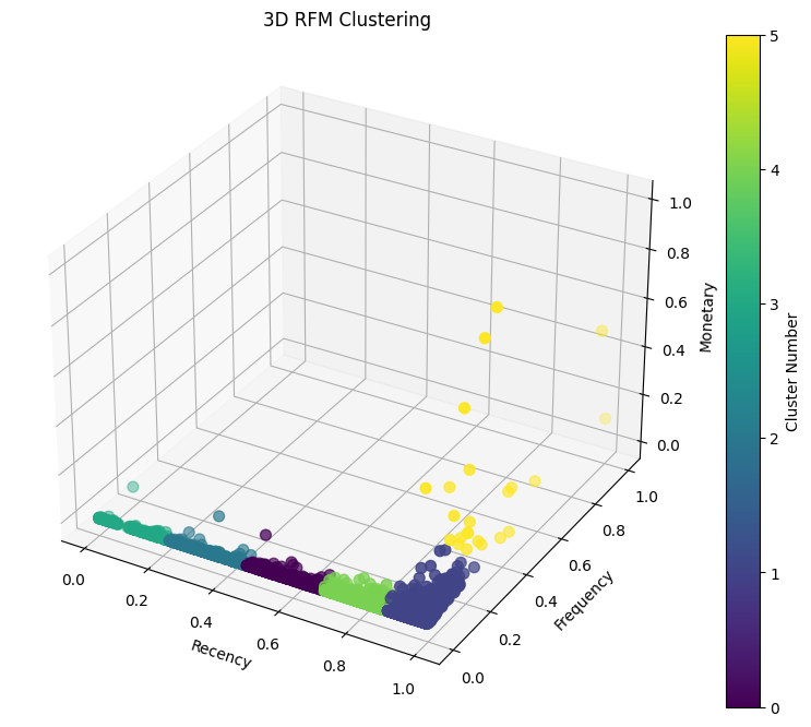
    km_final = KMeans(n_clusters=6)
    km_final = km_final.fit(df_rfm_clustering.drop("CustomerID", axis=1))
    df_rfm_clustering["cluster_number"] = km_final.predict(df_rfm_clustering.drop("CustomerID", axis=1))
Conclusion
In this E-commerce Customer Action Analysis project, we employed the RFM (Recency, Frequency, Monetary) method to gain insights into customer behavior and classify customers based on their characteristics. The analysis involved using Python and various libraries such as Pandas, Numpy, SKlearn, and Matplotlib.
Key Findings
1. Dataset Overview:
- The dataset, sourced from the UCI Machine Learning Repository, provided transactional data for a UK-based online retail store specializing in unique all-occasion gifts.
- Key variables included
InvoiceNo,StockCode,Description,Quantity,InvoiceDate,UnitPrice,CustomerID, andCountry.
2. Exploratory Data Analysis (EDA):
- Pandas-profiling and custom EDA techniques were employed to understand the dataset’s structure, distribution, and patterns.
- Data cleaning steps included handling duplicated values, addressing outliers, and casting columns to the appropriate data types.
3. Feature Engineering:
- Recency, Frequency, and Monetary features were engineered to quantify customer behavior.
- N-tile calculations were applied to categorize customers into segments based on their Recency, Frequency, and Monetary scores.
- Min-max scaling was performed to standardize the features for clustering.
4. Heuristic RFM Analysis:
- A heuristic approach was used to analyze customer segments, identifying VIP customers and those with changing purchasing patterns.
- Special attention was given to customers who had made frequent purchases in the past but had reduced their buying activity recently.
5. K-means Clustering:
- K-means clustering was applied to group customers based on their RFM scores.
- The Elbow Method was used to determine the optimal number of clusters, leading to the selection of
k=6. - The resulting clusters provided a segmentation of customers with similar purchasing behavior.
Business Implications
1. Customer Segmentation:
- The identified clusters can guide targeted marketing strategies tailored to the specific needs and preferences of each customer segment.
- Understanding the distinct behaviors of VIP customers and those with changing patterns allows for personalized engagement approaches.
2. Operational Improvements:
- Insights into purchase trends by day, month, and hour can inform inventory management and staffing decisions.
- Identifying countries with high and low purchase rates may guide international expansion strategies.
3. Future Work:
- Continuous monitoring and updating of customer segments based on changing trends and preferences.
- Integration of machine learning models for predictive analytics, such as forecasting future purchases and customer churn.
In conclusion, this analysis provides valuable insights for optimizing marketing strategies, improving customer experience, and making data-driven business decisions in the dynamic landscape of e-commerce.